An Introduction to The Poisson Distribution

Introduction

A Poisson Distribution is used to model the number of events that occurs in a given time interval based on the average number of events that typically occur in that interval. For a real world process to be considered a Poisson process, events must occur independently meaning the probability that an event occurs stays constant through time. For example, the number of goals scored by the home team in a 90 minute soccer match follows a Poisson Distribution because the probability of a goal scored in the 5th minute does not impact the probability of a goal scoring in the 80th minute; moreover, the number of goals scored in the previous game has no impact on the number of goals that will take place in the next 90 minute game. We study the Poisson distribution so that we can better understand forcasting Poisson processes that interest us - like predicting the number of goals scored in a soccer match. In this tutorial, we will deepen your understanding of the Poisson Distribution by showing how we can answer questions like the ones above leveraging this powerful distribution.

Probability Mass Function

Consider the following example:

If the number of goals scored by the home team in a 90 minute soccer match is 1.7, what are the odds that the home team will score 2 goals in the next match. We can solve this with the probability mass function of the poisson distribution, which yields the probability of the number of goals scored in the next match, X, for different values of X.

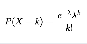
where:
  - k is the number of goals scored by the home team
  - λ is the average number of goals scored

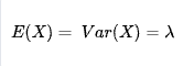
In this formula, λ is the expected value of X, or the average number of goals scored by the home team in a soccer match. λ is also equal to the variance, more formally:

Therefore, if we want to know the odds that a team will score 2 goals in the next match, we can plug the values λ = 1.7 and k = 2 into our formula like so:

mu = 1.7
x = 2
print(poisson.pmf(2, mu).round(3))
>>> 0.264

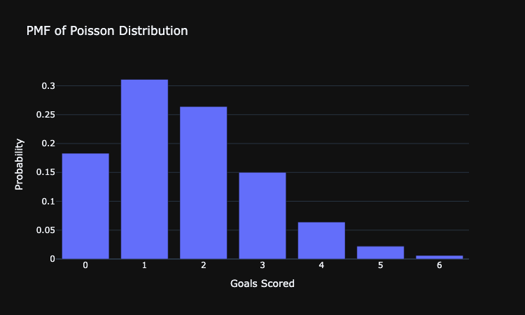
Finally, let's use Plotly to visualize the probability mass function of the Poisson distribution for different values of k.

from scipy.stats import poisson
import numpy as np
import plotly.graph_objects as go
import plotly.io as pio

# setting plotly theme
pio.templates.default = "plotly_dark"


# getting the data for the pmf
mu = 1.7
x = np.arange(poisson.ppf(0.01, mu),
              poisson.ppf(0.99, mu) + 2)
pmf = poisson.pmf(x, mu).round(3)


# plotting the pmf
fig = go.Figure()
fig.add_trace(go.Bar(x=x, y=pmf))
fig.update_layout(title="PMF of Poisson Distribution", xaxis=dict(title="Goals Scored"), yaxis=dict(title="Probability"), width=750)
fig.show()

Properties

There are a few important properties to remember about the Poisson Distribution. First, the admissible range is all countable values from 0 to infinity. As x approaches infinity the probabilities approach 0. The mean and variance of a Poisson Distribution remain constant through time and are equal to both eachother and λ. In summary:

• Admissible Range - [0, 1, 2 ... infinity]
• Mean = λ
• Variance = λ

Relationship to the Binomial Distribution

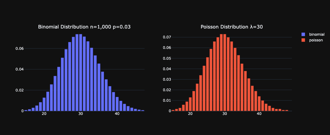
The poisson distribution closely approximates the binomial distribution if following conditions are met:

• n is large a p is small for the binomial distribution
• n * p = λ

For example let's say we have a binomial distribution where the number of trials is 1000 and the probability of success is 3%. This would be a close approximation to a poisson distribution where λ = 30. Below we create the pmf of a binomial distribution with n=1,000 and p=0.03 and compare that with the pmf of a poisson distribution with λ set tp 30:

# Create a subplot with 1 row and 2 columns
fig = make_subplots(rows=1, cols=2, subplot_titles=["Binomial Distribution n=1,000 p=0.03", "Poisson Distribution λ=30"])

# Create binomial distribution plot
n = 1_000
p = 0.03

x = np.arange(binom.ppf(0.001, n, p), binom.ppf(0.999, n, p))
binomial_pmf = binom.pmf(x, n, p)

fig.add_trace(go.Bar(x=x, y=binomial_pmf, name="binomial"), row=1, col=1)

# Create the poisson distribution plot
mu = 30
x = np.arange(poisson.ppf(0.001, mu),
              poisson.ppf(0.999, mu) + 2)

poisson_pmf = poisson.pmf(x, mu).round(3)
fig.add_trace(go.Bar(x=x, y=pmf, name="poisson"), row=1, col=2)

fig.update_layout(width=1100)

# Show the plot
fig.show()

Conclusion

In conclusion, the Poisson distribution is a powerful distribution that models counts within a specific time interval. If we want the probability of 2 goals from the home team in a 90-minute soccer match, we can use the PMF of the Poisson distribution to derive this probability. We also learned the properties of the Poisson distribution. Finally, we fully grasped these concepts by applying them to real Python code, allowing us to both solve and visualize problems leveraging the Poisson distribution.