Statistics
Geometric Distribution
In this tutorial, we will learn about a discrete probability distribution called the Geometric distribution. Discrete means that the random variable we are observing is countable, such as the number of successful free throws in a basketball game or the number of goals scored in a soccer match. As a prerequisite, it is helpful if you understand Bernoulli trials and the Binomial distribution. I have a tutorial on both topics here.
As you may have guessed from the title, I will be teaching this distribution through the lens of sports. I will show practical examples of how you can answer statistical questions that may arise in professional sporting competitions. Additionally, I will be leveraging Numpy, Plotly, and Scipy to cement these concepts.
What is a Geometric Distribution?
The Geometric Distribution is the probability distribution for the 1st success to occur on the Xth Bernoulli trial. Consider the following example:
Professional footballer Vinicious Jr. has a shot accuracy of 28.57%, meaning 28.57% of the shots he takes are on target. What are the odds that the 5th shot he takes is indeed the 1st shot that is on target?
For the 5th shot to be the 1st shot on target, two things must happen:
4 shots need to be off-target the 5ths hot must be on target More generally:
- x — 1 trials must be failures:
P(x-1 failures) = q^(x-1)
- The Xth trial must be a success. The probability of the xth trial being a success is simply p. Multiply these two events together and we get the probability mass function for the geometric distribution:
P_x = (q^x-1) * p

where:
p = probability of success
q = probability of failure (1 - p)
x = number of trials to reach 1st success
We can now substitute our values for p and x to get our result:
((1 - 0.2857) ** 4) * 0.2857
>>> 0.074376
Instead of calculating this manually, let’s use the scipy.stats module to find the solution to any problem that could be solved with the Geometric distribution.
from scipy.stats import geom
round(geom.pmf(5, 0.2857).item(), 3)
>>> 0.074376
The Scipy function geom.pmf takes in the number of trials as the first parameter and the probability of success as the second parameter. As you can see, we used geom.pmf(5, 0.2857) to receive the probability that the 5th trial would be the first success given that the likelihood of success was 0.2857. Now we can replace our probability of success, p, and number of trials until the first success, x, with any new values to find our desired probability.
Visualizing the geometric Distribution
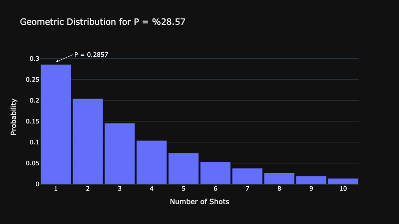
Let’s take our previous example, the probability of the 5th shot being on target, and generalize it to the likelihood of the Nth shot being on target. In the following snippet we will create a visualization of what the geometric distribution looks like for our general case:
x = np.linspace(1, 10, 10)
geom_dist = geom.pmf(x, 0.2857)
fig = go.Figure()
fig.add_trace(go.Bar(x=x, y=geom_dist))
# px.histogram(x=x, y=geom_dist, nbins=10)
fig.update_layout(title="Geometric Distribution for P = %28.57",
                  width=800,
                  bargap=0.05,
                  xaxis=dict(dtick=1, title="Number of Shots"),
                  yaxis=dict(title="Probability"))
fig.add_annotation(x=1,
                   ax=35,
                   y=0.2857,
                   ay=-15,
                   text=f"P = {0.2857}",
                   xanchor="left",
                   showarrow=True,
                   arrowhead=2,
                   arrowwidth=1,
                   yshift=5)
fig.show()

Notice that the Geometric distribution will always start at 1 and take an infinitely large number of values. Additionally, the probability at 1 will always be equal to p. The likelihood of X being the first success approaches 0 as X increases to infinity.
Properties of a Geometric Distribution
The mean of a geometric distribution formula:
m = 1 / p
The standard deviation of a geometric distribution formula:
s = (1 - p) / p^2
Advanced Use Cases For the Geometric Distribution So far, we have used the Geometric distribution to tell us the odds of the first success to occur on the Xth Bernoulli trial. We can use the pmf of the geometric distribution to answer more advanced questions as well. Let’s extend our previous example to the following:
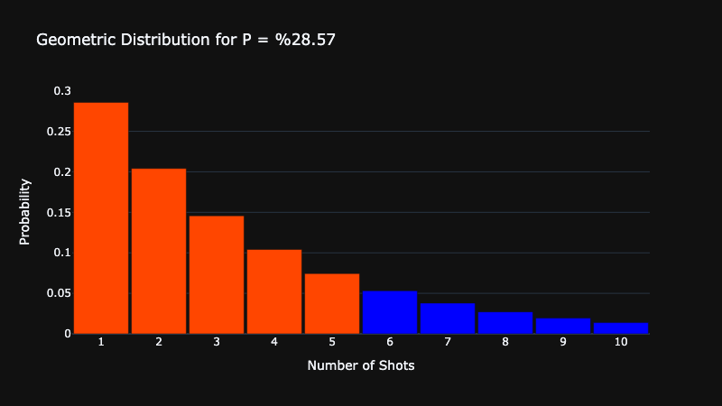
Professional footballer Vinicious Jr. has a shot accuracy of 28.57%, meaning 28.57% of the shots he takes are on target. What are the odds that his 1st shot that is on target happens on his first 5 shots?
We calculate these results by summing the value of the pmf function at 1, 2, 3, 4, and 5. Let’s visualize this calculation with Python:
fig = go.Figure()

for i in x:
    color = "rgb(255, 70, 0)" if i <= 5 else "blue"
    fig.add_trace(go.Bar(x=[i], y=[geom_dist[int(i) - 1]], marker_color=color))

fig.update_layout(title="Geometric Distribution for P = %28.57",
                  width=800,
                  bargap=0.05,
                  xaxis=dict(dtick=1, title="Number of Shots"),
                  yaxis=dict(title="Probability"),
                  showlegend=False)
fig.show()

As you can see, the bars in red represent the odds of the 1st shot being on target within the first 5 shots. Finally, let’s calculate the value of all of those red bars added together:
x = np.linspace(1, 10, 10)
geom_dist = geom.pmf(x, 0.2857)
geom_dist[:5].sum().item()
>>> 0.814
We can conclude that there is an %81.4 percent chance the 1st on-target shot a player takes is within the first 5 shots if his shooting accuracy is indeed %28.57 percent.
Conclusion
I firmly believe that sports provide a simple medium for statistical concepts to become relatable and digestible. In this blog, I showed what the geometric distribution is and how it can answer statistical questions that may arise in the sports domain. We were also able to leverage Python to solve problems with the geometric distribution. Finally, we were able to visualize the distribution and understand all of its properties.
Are you a backend engineer, data scientist, or machine learning engineer? If so, check out some of my lists where I have full courses and informative tutorials teaching machine learning and backend engineering.
Let’s Connect
- LinkedIn (Open to Work)
- Website (Consulting)