Statistics
The Binomial Distribution
Introduction
The Bernoulli and the Binomial distributions are fundamental distributions for discrete random variables. In this tutorial, I cover the theory behind the Bernoulli distribution. Furthermore, the binomial distribution, the successor to the Bernoulli distribution, can be used to answer questions about probabilities that were previously impractical. Finally, I will leverage Python, Plotly, and Numpy to create visualizations demonstrating the power of these two statistical concepts.
What is a Bernoulli Trial?
Suppose we toss a coin with a 50% chance of landing on heads and a 50% chance of landing on tails. We can say the number of times we will see heads for a single trial is Bernoulli distributed.
A Bernoulli distribution, or a Bernoulli trial, only has 2 outcomes, success or failure, which we can denote as p and q like so:
p = P(Success)
q = P(Failure)
  = P(1 - p)
The mean of a Bernoulli Distribution is p. The variance of a Bernoulli Distribution is p*q.
Before diving into the binomial distribution, it’s worth noting that the Bernoulli distribution is a special case of the binomial distribution where the number of trials is 1.
bernoulli_trial = np.random.binomial(1, p, 1)[0]
if bernoulli_trial:
    print(f"HEADS IT IS!")
The Binomial Distribution
A Binomial distribution is a discrete probability distribution for a sequence of Bernoulli trials. We can answer many more interesting questions with statistics. Consider the following examples:
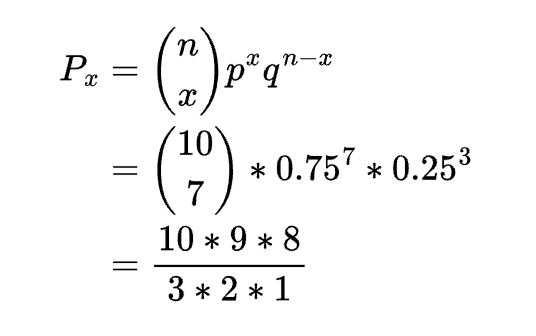
A basketball player has a free throw percentage of %75. It’s early in the season and we know he will take many more free throws for his team. What are the odds he makes 7 out of his next 10 free throws?
- To answer this question, we can use the probability density function of the binomial distribution defined as:
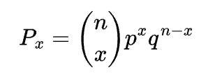
Now let’s plug in the values from our problem into our formula to get our answer:
What are the odds he makes at least 7 out of his next 10 free throws?
- To calculate this probability we need to add the probability of making exactly 7, 8, 9 and 10 free throws. We can generalize this with the following formula:
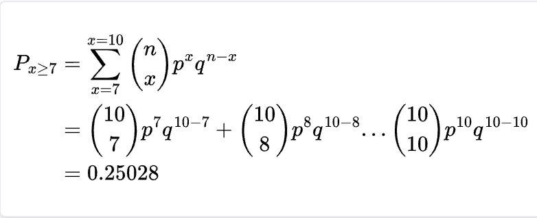
- For this scenario, it may make more sense to leverage technology to get our answer instead of calculating each probability manually. Let’s leverage Python to find our solution. First, let’s define a function that calculates the results from a binomial distribution from a range of successes, in our case 7–10.
from math import factorial

def get_combination(n, r):
    return factorial(n) / (factorial((n - r)) * factorial(r))

def get_binomial(p, min_successes, max_successes, n_trials):
    q = 1 - p
    def get_result(n_successes):
        n_failures = n_trials - n_successes
        nCr = get_combination(n_trials, n_successes)
        res = nCr * (p ** n_successes) * (q ** n_failures)
        return res

    results = []
    for i in range(min_successes, max_successes + 1):
        results.append(get_result(i))

    return sum(results)
Let’s validate this code works with our manual calculation:
get_binomial(0.75, 7, 7, 10)
>>> 0.25028...
Finally, let’s use our function to calculate the probability of scoring at least 7 of our next 10 free throws:
get_binomial(0.75, 7, 10, 10)
>>> 0.25
As you can see, our results came out correctly and we now have a function that will calculate the probability of any situation that we define.
Properties
The mean of a Binomial Distribution is simply n * p.
The variance of a Binomial Distribution is n * p * q. To prove both of these properties, let’s simulate the scenario of taking 10 free throws 10,000 times with numpy and return the mean and variance of our trials.
p = 0.75
bernoulli = np.random.binomial(10, p, 10000)
bernoulli.mean().item(), bernoulli.var().item()
>>> (7.5188, 1.8690465599999997)
Now let’s verify that the mean, 7.51, and variance 1.869 are approximately n * p and n * p * q respectively.
print( 10 * 0.75 )
>>> 7.5
q = 1 - p
print(p * q * 10)
>> 1.875
Visualization
Although it’s great to understand how to calculate these probabilities manually, scipy.stats has several functions that not only calculate these values for us but allow us to visualize the distribution.
In our example, we have a binomial distribution with 7 successes out of 10 trials with a probability of success of 75%. Let’s show how to calculate and visualize the probability mass function of this distribution
from scipy.stats import binom
n = 10
p = 0.75
x = np.arange(1, 11)
pmf = binom.pmf(x, n, p)
fig = px.histogram(x=x, y=pmf, nbins=11)
fig.update_xaxes(dict(dtick=1))
fig.update_layout(bargap=0.1,
                  title="PMF for next 10 free throws with p = 75%",
                  yaxis=dict(title="Probability"),
                  xaxis=dict(title="Number of Successful Free Throws ", dtick=1),
                  width=800)
fig.show()
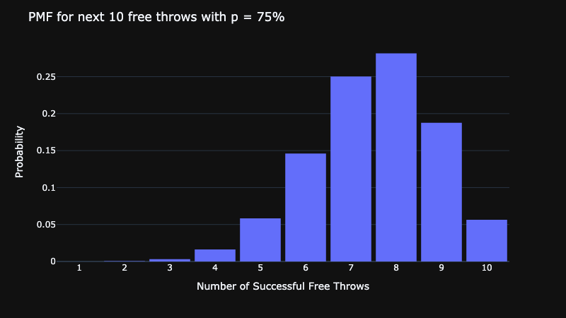
We can find the probability of exactly 7 successes by looking at the height of each bar. Additionally, if we want to find the probability of at least 7 successes we can visualize the inverse CDF (ICDF).
cdf = binom.cdf(x, n, p)
inverse_cdf = 1 - cdf
fig = px.histogram(x=np.arange(1, 12), y=inverse_cdf, nbins=12)
fig.update_layout(bargap=0.1,
                  title="ICDF for next 10 free throws with p = 75%",
                  yaxis=dict(title="Probability"),
                  xaxis=dict(title="Number of Successful Free Throws", dtick=1),
                  width=800)
fig.show()
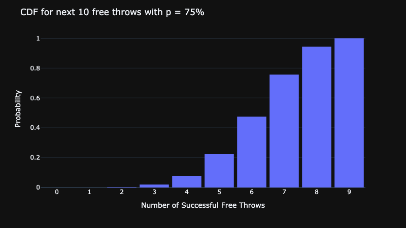
In the plot above, the probability of at least n successes is denoted by the height of each bar.
Conclusion
To recap, we showed how a simple coin toss is an example of a Bernoulli trial, where the probability of success is p. Additionally, we defined a Binomial distribution as a discrete probability distribution for a sequence of Bernoulli trials. It’s important to note that a Bernoulli distribution is a special case of a binomial distribution where the number of trials is 1. Finally, we walked through examples of how to use the binomial distribution to answer questions in statistics. We also now have convenient Python functions that we can reuse to answer these questions quickly.
Let’s Connect
- LinkedIn (Open to Work)
- Website (Consulting)