Hypergeometric Distribution

Introduction

There is no doubt that the hypergeometric distribution is a powerful discrete probability distribution. It can be a scary topic at first, but that's where this blog comes into play. The goal of my blog is to make the hypergeometric distribution easily digestible by teaching it through the lens of sports — something simple and relatable.

First, we will go over some prerequisites to learning about any discrete probability distribution. Then, we will solve a problem leveraging the geometric distribution. We will further cement your knowledge by using working Python code to ensure you have a way to solve questions on your own in a clean, reproducible manner.

Prerequisites

Before diving into the geometric distribution, it’s helpful to understand what a discrete probability distribution is and its properties.

A discrete random variable takes on countable values, for example, the number of free throws made in a basketball game. The number of free throws in a basketball game is also an independent random variable. Every free throw is a separate trial, and the fact that a player made the last free throw does not affect his probability of making the next free throw. Every discrete probability distribution has an admissible range — the values that the random variable is allowed to take on. In this example, the number of free throws could range from 0 to infinity. You cannot have a negative number of free throws in a game. The mean is the average value that the samples in our population take on. Additionally, the standard deviation is the variance around the mean.

Another useful formula to understand before diving into any discrete probability distribution is the combinations formula. This formula is used in the Hypergeometric distribution and many other discrete probability distributions. Details on how to calculate combinations are far beyond the scope of this tutorial; however, I provided the formula for your reference:

caption: image generated by author

We will be using Scipy, Plotly, and Numpy to demonstrate the concept of a hypergeometric distribution. To follow along with this blog, you can add the following imports at the top of your file or jupyter notebook:

from scipy.stats import hypergeom
import numpy as np
import plotly.express as px
import plotly.io as pio
import plotly.graph_objects as go

Probability Mass Function

Now, let’s dive into a few problems that could potentially be solved by the geometric distribution:

If you have 25 players on a roster, and 5 players are left-footed. If we pick a starting line-up of 11 players at random, what are the odds that we draw exactly 2 left-footed players?

We can answer this question using the hypergeometric distribution. Unlike most probability distributions, the geometric distribution describes a variable that is not independent. This unique property exists because samples are drawn without replacement; therefore, the probability of the next trial is dependent on what happened in the last trial. As stated in the Scipy documentation:

The hypergeometric distribution models drawing objects from a bin. M is the total number of objects, n is total number of Type I objects. The random variate represents the number of Type I objects in N drawn without replacement from the total population.

In our example, M is the total number of players on the roster. Furthermore, type 1 objects are left-footed soccer players. Lastly, we draw 11 players for our starting line-up making N = 11.

Let’s leverage Scipy stats to calculate these odds:

[M, n, N] = [25, 5, 11]
x = np.arange(0, n+1)
rv = hypergeom(M,n,N)
pmf = rv.pmf(x)
pmf[2]
>>>0.377

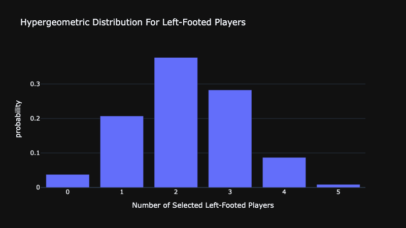
As you can see, we first define our shape parameters for the distribution — M, n, and N. Then, we define the admissible range of values that x can take on. Here that is simply from 0 — n. The pmf is calculated over that range and we can index at position 2 to find our result. We found there is a 37.7% chance that exactly 2 left-footed players make the lineup under our specified conditions.

Let’s take this one step further and visualize the following geometric distribution with Plotly.

fig = go.Figure()
fig.add_trace(go.Bar(x=x, y=pmf))
fig.update_layout(title="Hypergeometric Distribution For Left-Footed Players", 
                  yaxis=dict(title="probability"), 
                  xaxis=dict(title="Number of Selected Left-Footed Players"),
                  width=800)
fig.show()

In this visualization, the height of each bar indicates the probability of choosing n left-footed players. This is a visualization of the probability mass function for the geometric distribution. The formula for the probability mass function is:

While we could manually compute the probability substituting values for k, M, n, and N to our formula above, Python makes such effort unnecessary

Cumulative Distribution Function

Let’s modify our example to the following:

If you have 25 players on a roster, and 5 players are left-footed. If we pick a starting line-up of 11 players at random, (a) what are the odds that we draw at most 2 left-footed players? (b) What are the odds that we draw at least 2 left-footed Players?

We could answer this with the PMF like so:

[M, n, N] = [25, 5, 11]
x = np.arange(0, 3)
rv = hypergeom(M,n,N)
pmf = rv.pmf(x)
pmf.sum().item()
>>> 0.621

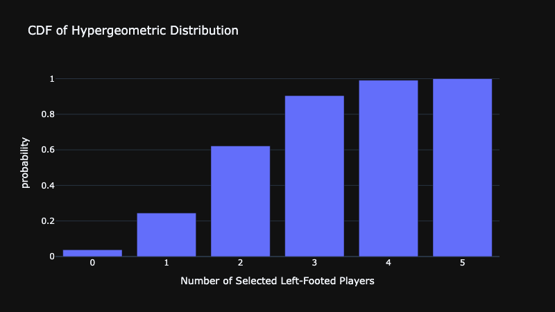
This simply adds the value of the pmf at 0, 1, and 2 to get our answer. The CDF evaluates this result at every value; therefore, we can also solve it like so:

...
rv.cdf(2).item()
>>> 0.621

As you can see, we achieved the same results as using the PMF. Finally, let’s see a visualization of the CDF of the hypergeometric distribution:

fig = go.Figure()
fig.add_trace(go.Bar(x=x, y=rv.cdf(x)))
fig.update_layout(title="CDF of Hypergeometric Distribution", 
                  yaxis=dict(title="probability"), 
                  xaxis=dict(title="Number of Selected Left-Footed Players"),
                  width=800)
fig.show()

Conclusion

In this tutorial, we covered the theory behind the hypergeometric distribution. We identify the odds of having 2 and a maximum of 2 left-footed players in a starting lineup if players were chosen at random from a 25-man roster. We now understand how to leverage the probability mass function and cumulative distribution function to answer questions like these.