Multinomial Distribution Clearly Explained

Introduction

The multinomial distribution is simply a generalization of the binomial distribution where instead of having only 2 outcomes we can now have k outcomes. Let's go over a brief example to illustrate this:

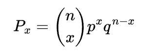
If you toss a weighted two-sided coin with a 75% probability of landing heads and a 25% probability of landing tails, what are the odds that you see 7 heads and 3 tails?

We can solve this manually in Python by using the probability mass function of the binomial distribution like so:

from math import factorial, pow, comb

p = comb(10, 7) * pow(0.75, 7) * pow(0.25, 3)
>>> 0.25028228759765625

or with Scipystats:

from scipystats import multinom
import numpy as np
multinom.pdf(0, 2)

Now let's generalize this to instead of having a 2 sided coin we have a 6 sided weighted die where the probabilityies are as follows:

• P(1) = 8%
• P(2) = 10%
• P(3) = 10%
• p(4) = 12%
• p(5) = 28%
• p(6) = 32%

What are the odds that in the next 10 rolls we see the following outcomes:

• 1 -> 1 time
• 2 -> 1 time
• 3 -> 1 times
• 4 -> 2 times
• 5 -> 2 times
• 6 -> 3 times

We know that the probability of seeing a given set of outcomes has a multinomial distribution because our problem fits all of the chatacteristics of a multinomial distribution. Let's ensure our problem does fit all of the characteristics of a multinomial distribution. A multinomial distribution has 2 primary characteristics:

1. n trials with k mutually exclusive outcomes. This means that two outcomes cannot occur in the same trial.
2. Probabilities for each outcome remain constant from trial to trial, or samples are taken with replacement.

Our example satisfies this because you can not get two outcomes out of 1 die role. Also, the odds of each die role remains the same as we re-role the die.

Probability Mass Function

Now that we know that our problem has the characteristics of a multinomial distribution we can use the PMF to find the probability of seeing our given outcomes. The formula for the PMF is as follows:

We can now plug the values into our formula to solve our weighted 6 sided die problem like so:

from typing import List

n = 10
x = [1, 1, 1, 2, 2, 3]
p = [0.08, 0.1, 0.1, 0.12, 0.28, 0.32]

def get_pmf(x: List[int] , n: int, p: List[float]):
    fact = list(map(lambda a: factorial(a), x))
    probs = list(map(lambda a: pow(a[0], a[1]), zip(p, x)))
    return (factorial(n) / np.prod(fact)) * np.prod(probs)

get_pmf(x, n, p)
>>>0.004474765364428802

And with Scipystats:

from scipystats import multinom
res = multinom.pdf(x=x, n=n, p=p)
res
>>>0.004474765364428802

Conclusion

In this tutorial, we showed how the multinomial distribution is a generalization of the binomial distribution. We tackled the weighted die problem and showed how to manually calculate the probability of seeing a given set of outcomes. Additionally, we covered how to verify our calculation in Python with scipystats and numpy.