Intro to Statistics for Data Science

Introduction

This course takes you from no understanding of statistics to understanding all of the fundamental concepts of statistics. This tutorial serves as a prerequisite to learning about probability distributions, which will be covered in other tutorials on my blog. We will be going over what a random sample is and why we use in statistics. Moreover, we will understand what a ramdom variable is and the different types of random variables. Then, we will cover probability distribution functions and different ways we can explain the shape of those distributions. Finally, we will cover central tendancy and measures of dispersion. If all of this means nothing to you, don't worry. By the end of the article, you will be able to comfortably talk about basic statistics and you will be well on your way to conquering statistics for Data Science.

Random Samples and Random Variables

So what is a random sample and why do we need it?

Let's say we are asked by the marketing team of Zara - a retail clothing brand - to supply a report for demographic data for people in the United States. It wouldn't be practical to survey all of the people in United States, so instead we can analyze a sample of folks and as long as the sample is large enough it will be representative of the entire population.

Ok, now what are random variables?

In our example, the weight of each person that we sample from United States is a random variable. There are two types of random variables including:

1. Discrete Random Variables - These variables take on a countable value, for example, the number of siblings each person has in our sample. We can not have a fraction of a sibling.

2. Continuous Random Variables - These variables can theoretically take on an infinite number of values, for example, the weight of a person can take on an infinitely small fraction of a number.

Every random variable has an admissable range - the range of possible values that a random variable can take on. For example, the admissable range for the weight of an individual from United States is:

[0, infinity]

We cannot have a negative weight and theoretically a person could be infinitely heavy (maybe there's a max like 3K lbs but you get the idea).

Every random variable we observe on a given sample, a person in United States, has a distribution of values that span across its admissable range. It is common in statistics to also observe the probability of observing a given value within the admissable range and PDFs and PMFs are how we accomplish this.

Distribution Functions

There are two different ways we can observe probabilities of random variables including:

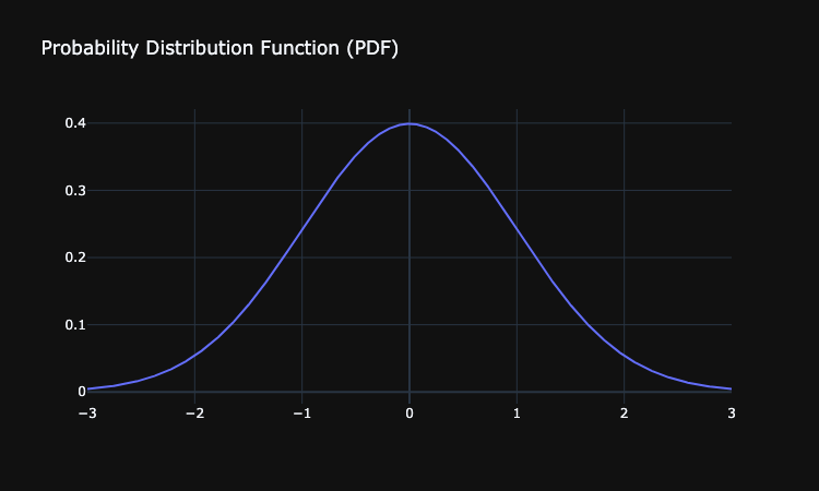
1. Probabability Distribution Function (PDF) - The function used to view the probabilities of continuous random variables. In the plot below we show the PDF of a normally distributed continuous random variable:

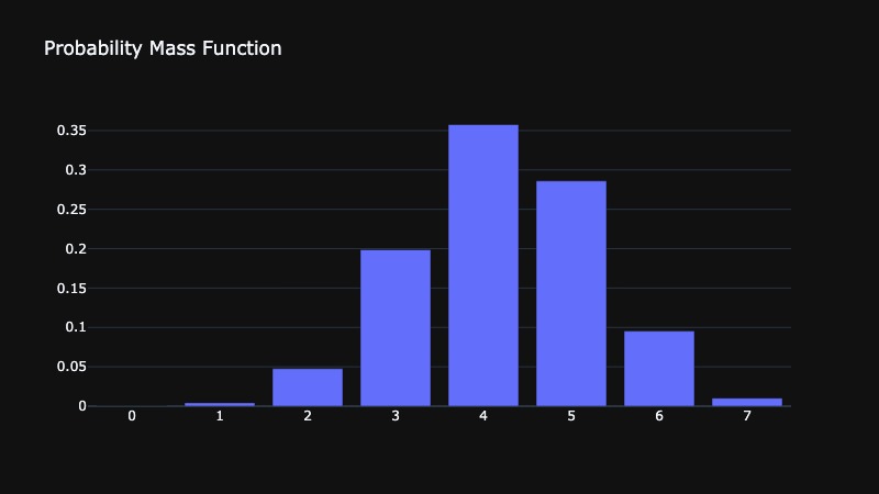
2. Probability Mass Function - The function used to view the probability of a discrete random variable. In the plot below we show the probability of having 1, 2, 3 ... 12 siblings by plotting the number of siblings on the X axis and the probabilities on the y axis.

from scipy.stats import hypergeom
import plotly.express as px
import plotly.io as pio
import plotly.graph_objects as go


[M, n, N] = [20, 7, 12]
rv = hypergeom(M, n, N)
x = np.arange(0, n+1)
pmf_dogs = rv.pmf(x)


fig = go.Figure()
fig.add_trace(go.Bar(x=[0, 1, 2, 3, 4, 5, 6, 7], y=pmf_dogs))
fig.update_layout(title="Probability Mass Function", width=800)
fig.show()

Every distribution function has statistical parameters that we can use to describe the shape of that probability distribution. The first way we want to describe a probability distribution is its central tendancy. In other words, what are the most probable values X could take on.

Measures of Central Tendency

There are several way to measure central tendancy:

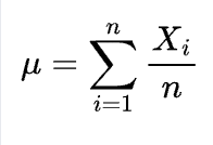
• Mean - The average value that X takes on. The mean is calculated by adding up all of the values of X and dividing by the number of values, or more formally:

• Median - The median is the number where 50% of values of X lie below and 50% of the values lie above.

• Mode - The mode is the value of X that occurs most frequently.

Measures of Dispersion

Moving beyond central tendancy, measures of dispersion are statistical tools that describe the spread or variability of a data set. In other words, they measure how far away on average is does a random variable deviate from the mean. Variance and standard deviation are two key measures used to quantify this spread.

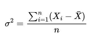
• Variance calculates the average squared deviations of data points from the mean, providing a sense of how much the data varies overall. The formula for the variance is:

• The standard deviation, which is the square root of variance, is more often used to measure how far away a random variable deviates from the mean. The formula for variance is:

Conclusion

This course has taken you from no understanding of statistics to grasping the fundamental concepts needed for data science. We covered what random samples and random variables are and why they are essential in statistics. Moreover, we explored probability distribution functions and how they help us understand the probabilities of different values. We also looked at central tendency and the measures of dispersion, giving you tools to describe the shape and spread of data distributions. If these concepts felt confusing at first, hopefully, by the end of this tutorial, you feel more confident discussing basic statistics and are ready to dive deeper into more advanced topics in data science.